Admin
مدير المنتدى


عدد المساهمات : 18726
التقييم : 34712
تاريخ التسجيل : 01/07/2009
الدولة : مصر
العمل : مدير منتدى هندسة الإنتاج والتصميم الميكانيكى
 |  موضوع: رسالة دكتوراة بعنوان Efficient Finite Element Modelling of Ultrasound Waves in Elastic Media السبت 22 أكتوبر 2022, 9:31 pm موضوع: رسالة دكتوراة بعنوان Efficient Finite Element Modelling of Ultrasound Waves in Elastic Media السبت 22 أكتوبر 2022, 9:31 pm | |
| 
أخواني في الله
أحضرت لكم
رسالة دكتوراة بعنوان
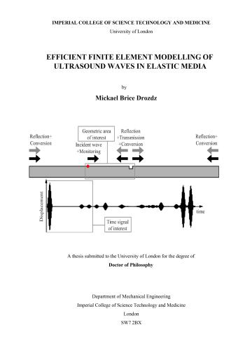
Efficient Finite Element Modelling of Ultrasound Waves in Elastic Media
by
Mickael Brice Drozdz
A thesis submitted to the University of London for the degree of
Doctor of Philosophy
IMPERIAL COLLEGE OF SCIENCE TECHNOLOGY AND MEDICINE
University of London
Department of Mechanical Engineering
Imperial College of Science Technology and Medicine
و المحتوى كما يلي :
Table of contents
Chapter 1
Introduction
1. Introduction . 18
2. Objectives 19
3. Outline of the thesis . 22
Chapter 2
Theoretical background
1. Introduction . 24
2. Theory of wave propagation in elastic media . 24
2.1 Bulk wave propagation 24
2.1.1 Bulk wave propagation in infinite isotropic elastic media 24
2.1.2 Bulk propagation in a semi-infinite isotropic elastic medium . 26
2.2 Guided wave propagation in a plate 28
3. Finite elements modelling of wave propagation . 34
3.1 Explicit method 35
3.2 Implicit method 37
3.2.1 ABAQUS/Standard procedure . 38
3.2.2 COMSOL Multiphysics procedure . 40
4. Conclusions . 42
Chapter 3
Modelling waves in unbounded elastic media using absorbing layers
1. Introduction . 43
2. Review of non-investigated techniques 45
2.1 Infinite element methods . 45
2.2 Non reflecting boundary condition . 47
3. Absorbing layer theory 47
3.1 Concept 47
3.2 Perfectly matched layer (PML) 48
3.3 Absorbing layer using increasing damping (ALID) 50
4. Efficient layer parameters’ definition . 53
4.1 Analytical model for bulk waves . 54
4.1.1 General definition 55
4.1.2 Validation procedure 55
4.1.3 PML analytical model . 57
4.1.4 ALID analytical model 61
4.2 Analytical model for 2D guided wave cases 66
4.2.1 Consideration for guided wave PML implementation 66
4.2.2 Validation procedure 67
4.2.3 PML analytical model for guided wave cases 68
4.2.4 ALID analytical model 71
5. Demonstrators . 77
5.1 Computational efficiency 77
5.1.1 Bulk wave model 77
5.1.2 Guided wave model 80Table of contents
7
5.2 Time reconstruction 81
5.3 Wave scattering 84
5.3.1 Single-mode reflection coefficient . 84
5.3.2 Multi-mode reflection coefficient 86
6. Discussion 88
7. Conclusion 89
Chapter 4
On the influence of mesh parameters on elastic bulk wave velocities
1. Introduction . 90
2. Explicit solving 91
2.1 Introduction . 91
2.2 Linear quadrilateral elements . 92
2.2.1 Square elements . 92
2.2.2 Rectangle elements 100
2.2.3 Rhombus elements 102
2.2.4 Parallelogram elements . 104
2.2.5 Conclusion 105
2.3 Linear triangular elements . 106
2.3.1 Equilateral triangle elements . 106
2.3.2 Isosceles triangle elements 110
2.3.3 Scalene triangle elements . 112
2.3.4 Conclusion 114
2.4 Modified quadratic triangular elements . 114
2.4.1 Equilateral triangle elements . 114
2.4.2 Isosceles triangle elements 119
2.4.3 Scalene triangle elements . 120
2.4.4 Conclusion 122
3. Implicit solving . 123
3.1 Introduction 123
3.2 Linear quadrilateral elements 123
3.2.1 Square elements 123
3.2.2 Rectangle elements 124
3.2.3 Rhombus elements 125
3.2.4 Parallelogram elements . 126
3.2.5 Conclusion 127
3.3 Quadratic quadrilateral elements 128
3.3.1 Square elements 128
3.3.2 Rectangle elements 129
3.3.3 Rhombus elements 130
3.3.4 Parallelogram elements . 131
3.3.5 Conclusion 132
3.4 Linear triangular elements . 133
3.4.1 Equilateral triangle elements . 133
3.4.2 Isosceles triangle elements 133
3.4.3 Scalene triangle elements . 134
3.4.4 Conclusion 135
3.5 Quadratic triangular elements 136
3.5.1 Equilateral triangle elements . 136
3.5.2 Isosceles triangle elements 137
3.5.3 Scalene triangle elements . 138Table of contents
8
3.5.4 Conclusion 139
3.6 Modified quadratic equilateral triangular elements 139
3.6.1 Equilateral triangle elements . 139
3.6.2 Isosceles triangle elements 140
3.6.3 Scalene triangle elements . 141
3.6.4 Conclusion 142
4. Conclusions 142
Chapter 5
Accurate modelling of defects using Finite Elements
1. Introduction 146
2. Model definition 148
3. Reflection from a straight edge . 150
4. Reflection from a straight crack at an angle . 156
4.1 Crack of unit length 158
4.2 Crack of length 0.25 . 161
4.3 Crack of length 4 165
4.4 Conclusion . 168
5. Reflection from circular defects 168
5.1 Hole of unit diameter . 170
5.2 Hole of diameter 0.25 173
5.3 Hole of diameter 4 . 176
5.4 Conclusion . 178
6. Conclusions 179
Chapter 6
Local mesh refinement
1. Introduction 181
2. Fictitious domain technique . 182
2.1 Review 182
2.2 Presentation 182
2.3 Conclusion . 183
3. Abrupt mesh density variation . 183
3.1 1D wave propagation models 183
3.1.1 Model definition 183
3.1.2 L wave 1D model using theoretical material properties 185
3.1.3 L wave 1D model with matched acoustic impedance 186
3.1.4 L and S wave 1D model with matched acoustic impedance . 187
3.1.5 L and S wave 1D model with varying acoustic impedance . 190
3.1.6 L wave 1D model with different mesh ratio . 193
3.2 2D wave propagation models 195
3.2.1 Model definition 195
4. Gradual mesh density variation . 199
4.1 1D wave propagation model . 199
4.2 2D wave propagation model . 201
5. Conclusions 202Table of contents
9
Chapter 7
Conclusions
1. Review of thesis 204
2. Summary of findings . 205
2.1 Absorbing layers 205
2.2 Influence of mesh parameters on the elastic bulk wave velocities 207
2.3 Accurate modelling of complex defects using Finite Elements 208
2.4 Local mesh refinement . 209
3. Future work 210
3.1 Absorbing layers 210
3.2 Influence of mesh parameters on the elastic bulk wave velocities 210
3.3 Accurate modelling of complex defects using Finite Elements 211
3.4 Local mesh refinement . 211
References10
List of figures
Figure 1.1 a) 2D plane strain model of a plate including a defect, b) Time signal at
the monitoring point 19
Figure 2.1 Modes considered and their orientation 25
Figure 2.2 Geometry of a 2D plate . 27
Figure 2.3 Typical deformation caused by symmetric (a) and anti-symmetric (b)
modes 28
Figure 2.4 Illustration of the deformation of a plate caused by a) propagating, b)
propagating evanescent, c) evanescent waves which have a) real, b) complex, c) imaginary wave numbers . 31
Figure 2.5 Phase velocity against frequency.thickness for a 3mm thick steel plate .
32
Figure 2.6 Wave number against frequency for a 3mm thick steel plate . 32
Figure 2.7 Example of S0 mode shapes for a free plate case at different frequencies
shown for a 3mm thick steel plate 33
Figure 2.8 Illustration of DL for a a) linear square element, b) linear triangle element
and c) quadratic triangle element 36
Figure 3.1 a) 2D plane strain model of a plate including a defect, b) Time signal at
the monitoring point 42
Figure 3.2 Illustration of use of infinite elements 44
Figure 3.3 ABAQUS benchmark model: a) Model geometry, b) vertical displacement at point A, Extended model (reference): c) Model geometry, d) vertical displacement at point A 45
Figure 3.4 Absorbing layer concept for 2D models: a) infinite medium, b) semi infinite medium, c) plate 46
Figure 3.5 Variation of αx(x) and αy(y) in a 2D model 48
Figure 3.6 Spatial spread of the reflection and transmission for a single layer (no
mode conversion shown for simplicity) 54
Figure 3.7 Illustration of extreme angles defining the range of angles to consider
when dimensioning an absorbing layer 54
Figure 3.8 FE model used to validate the analytical models a) normal incidence
model, b) angled incidence model 56
Figure 3.9 a) Reflection coefficient against αx b) Reflection coefficient against the
number of elements per wavelength . 57
Figure 3.10 Reflection coefficient for a given PML obtained with bulk wave analytical and FE models . 59
Figure 3.11 Reflection coefficient for a given ALID obtained with bulk wave analytical and FE models 64
Figure 3.12 FE model used to validate the guided wave analytical models 67
Figure 3.13 Reflection coefficient for a given PML obtained with guided wave analytical and FE models . 70
Figure 3.14 Definition of the multi layered system . 71
Figure 3.15 Reflection coefficient for a given ALID obtained with guided wave analytical and FE models . 76
Figure 3.16 a) bulk wave demonstrator, FE model: b) without absorbing layer, c) with
ALID, d) with PML 77List of figures
11
Figure 3.17 Absolute displacement field for the bulk demonstrator with ALID at
time: a)5msec b)10msec c)15msec d)20msec. Colour scale extends from
0 (blue) to 0.1% (red) of the maximum absolute displacement. Grey indicates out of scale (0.1% to 100%). White dashed line indicates the boundary between area of study and ALID 78
Figure 3.18 a) guided wave demonstrator, FE model: b) without absorbing layer, c)
with ALID, d) with PML 79
Figure 3.19 Absolute displacement field for the guided demonstrator with ALID at
time: a)150msec b)300msec c)450msec d)600msec. Colour scale is varied and extends from 0 (blue) to 2% or 10% (red) of the maximum absolute displacement as indicated on the figure. Grey indicates out of scale
(2% or 10% to 100%). White dashed line indicates the boundary between
area of study and ALID 80
Figure 3.20 Input preprocessing . 81
Figure 3.21 Model geometry for time reconstruction case 81
Figure 3.22 Normal displacement monitored 700mm away from the defect. a) Classical time domain analysis with ABAQUS, b) Frequency domain analysis
with ABAQUS, c) Frequency domain analysis with COMSOL 82
Figure 3.23 a) dispersion curve data used for input definition, b) input definition . 82
Figure 3.24 Representation of model used for guided wave scattering validation 83
Figure 3.25 Example of a typical spatial FFT curve 83
Figure 3.26 Reflection coefficient against notch width . 84
Figure 3.27 Energy reflection coefficient for A0 incident on a 2mm square notch in
an 8mm thick aluminium plate from 140kHz to 500kHz . 86
Figure 4.1 Definition of the main feature of the model . 90
Figure 4.2 a) Longitudinal and b) shear wave excitation for a square element mesh
and c) longitudinal and d) shear excitation for a triangular elements mesh
91
Figure 4.3 Schematic defining L0, L90, L45 and Lθ in a mesh of square elements .
92
Figure 4.4 a) Longitudinal and b) shear velocity errors against CFL for various mesh
densities at 0 degrees 93
Figure 4.5 Velocity error against mesh density for shear and longitudinal waves at 0
degree with a CFL of 0.025 95
Figure 4.6 Velocity errors against CFLX for various mesh densities at 0 degrees 95
Figure 4.7 Velocity error against mesh density for shear and longitudinal waves at 0
and 45 degree 97
Figure 4.8 Variation of the longitudinal (a and c) and shear (b and d) velocity error
against the angle of incidence for various values of mesh density plotted
in polar (a and b) and linear (c and d) plots 97
Figure 4.9 Velocity errors against CFLX for various mesh densities at 45 degrees .
98
Figure 4.10 Velocity error against the scaled Courant number CFLX and mesh density N . 99
Figure 4.11 a) Shape of the different rectangular elements used in the mesh; Variation
of the longitudinal (b and d) and shear (c and e) velocity error against the
angle of incidence for various R plotted in a polar (b and c) and linear (d
and e) fashion. The coloured circles indicate the error prediction along
the element side and diagonal . 100List of figures
12
Figure 4.12 a) Shape of the different rhombic elements used in the mesh; Variation of
the longitudinal (b and d) and shear (c and e) velocity error against the
angle of incidence for various shearing angle g plotted in a polar (b and
c) and linear (d and e) fashion. The coloured circles indicate the error prediction along the element side and diagonal . 102
Figure 4.13 a) Shape of the different parallelogramatic elements used in the mesh;
Variation of the longitudinal (b and d) and shear (c and e) velocity error
against the angle of incidence for various shearing angle g plotted in a polar (b and c) and linear (d and e) fashion. The coloured circles indicate the
error prediction along the element side and diagonal . 104
Figure 4.14 Schematic defining L0, L90, L30 and Lq in a mesh of equilateral-triangular elements . 105
Figure 4.15 Variation of the longitudinal (a and c) and shear (b and d) velocity error
against the angle of incidence for various mesh densities plotted in a linear (a and b) and polar (c and d) fashion 106
Figure 4.16 Velocity error against mesh density for shear and longitudinal waves at 0
and 30 degrees 107
Figure 4.17 Velocity errors against CFLX for various mesh densities at a) 0 and b) 30
degrees 108
Figure 4.18 a) Shape of the different isosceles-triangular elements used in the mesh;
Variation of the longitudinal (b and d) and shear (c and e) velocity error
against the angle of incidence for various values of f plotted in a polar (b
and c) and linear (d and e) fashion. The coloured circles indicate the error
prediction along the element side and diagonal 110
Figure 4.19 a) Shape of the different scalene-triangular elements used in the mesh;
Variation of the longitudinal (b and d) and shear (c and e) velocity error
against the angle of incidence for various values of g plotted in a polar (b
and c) and linear (d and e) fashion. The coloured circles indicate the error
prediction along the element side and diagonal 112
Figure 4.20 Variation of the longitudinal (a and c) and shear (b and d) velocity error
against the angle of incidence for various mesh densities plotted in a polar
(a and b) and linear (c and d) fashion . 114
Figure 4.21 Schematic defining L0, L90, L30 and Lq in a mesh of quadratic equilateral-triangular elements 114
Figure 4.22 Velocity error against mesh density for shear and longitudinal waves at 0
and 30 degrees 115
Figure 4.23 Velocity errors against CFLX for various mesh densities at a) 0 and b) 30
degrees 117
Figure 4.24 a) Shape of the different quadratic isosceles-triangular elements used in
the mesh; Variation of the longitudinal (b and d) and shear (c and e) velocity error against the angle of incidence for various values of f plotted
in a polar (b and c) and linear (d and e) fashion. The coloured circles indicate the error prediction along the element side and diagonal . 118
Figure 4.25 a) Shape of the different quadratic scalene-triangular elements used in the
mesh; Variation of the longitudinal (b and d) and shear (c and e) velocity
error against the angle of incidence for various values of g plotted in a polar (b and c) and linear (d and e) fashion. The coloured circles indicate the
error prediction along the element side and diagonal . 120
Figure 4.26 Variation of the longitudinal (a and c) and shear (b and d) velocity error
against the angle of incidence for various values of mesh density plotted
in linear (a and b) and polar (c and d) plots 123List of figures
13
Figure 4.27 a) Shape of the different rectangular elements used in the mesh; Variation
of the longitudinal (b and d) and shear (c and e) velocity error against the
angle of incidence for various values of R plotted in a polar (b and c) and
linear (d and e) fashion . 124
Figure 4.28 a) Shape of the different rhombic elements used in the mesh; Variation of
the longitudinal (b and d) and shear (c and e) velocity error against the
angle of incidence for various values of g plotted in a polar (b and c) and
linear (d and e) fashion . 125
Figure 4.29 a) Shape of the different parallelogramatic elements used in the mesh;
Variation of the longitudinal (b and d) and shear (c and e) velocity error
against the angle of incidence for various values of g plotted in a polar (b
and c) and linear (d and e) fashion 126
Figure 4.30 Variation of the longitudinal (a and c) and shear (b and d) velocity error
against the angle of incidence for various values of mesh density plotted
in polar (a and b) and linear (c and d) plots 127
Figure 4.31 a) Shape of the different rectangular elements used in the mesh; Variation
of the longitudinal (b and d) and shear (c and e) velocity error against the
angle of incidence for various values of R plotted in a polar (b and c) and
linear (d and e) fashion . 129
Figure 4.32 a) Shape of the different rhombic elements used in the mesh; Variation of
the longitudinal (b and d) and shear (c and e) velocity error against the
angle of incidence for various values of g plotted in a polar (b and c) and
linear (d and e) fashion . 130
Figure 4.33 a) Shape of the different parallelogramatic elements used in the mesh;
Variation of the longitudinal (b and d) and shear (c and e) velocity error
against the angle of incidence for various values of g plotted in a polar (b
and c) and linear (d and e) fashion 131
Figure 4.34 Variation of the longitudinal (a and c) and shear (b and d) velocity error
against the angle of incidence for various mesh densities plotted in a linear (a and b) and polar (c and d) fashion 132
Figure 4.35 a) Shape of the different quadratic isosceles-triangular elements used in
the mesh; Variation of the longitudinal (b and d) and shear (c and e) velocity error against the angle of incidence for various value of f plotted in
a polar (b and c) and linear (d and e) fashion . 133
Figure 4.36 a) Shape of the different scalene-triangular elements used in the mesh;
Variation of the longitudinal (b and d) and shear (c and e) velocity error
against the angle of incidence for various values of g plotted in a polar (b
and c) and linear (d and e) fashion 134
Figure 4.37 Variation of the longitudinal (a and c) and shear (b and d) velocity error
against the angle of incidence for various mesh density plotted in a linear
(a and b) and polar (c and d) fashion 135
Figure 4.38 a) Shape of the different quadratic isosceles-triangular elements used in
the mesh; Variation of the longitudinal (b and d) and shear (c and e) velocity error against the angle of incidence for various values of f plotted
in a polar (b and c) and linear (d and e) fashion . 136
Figure 4.39 a) Shape of the different scalene-triangular elements used in the mesh;
Variation of the longitudinal (b and d) and shear (c and e) velocity error
against the angle of incidence for various values of g plotted in a polar (b
and c) and linear (d and e) fashion 137List of figures
14
Figure 4.40 Variation of the longitudinal (a and c) and shear (b and d) velocity error
against the angle of incidence for various mesh densities plotted in a linear (a and b) and polar (c and d) fashion 138
Figure 4.41 a) Shape of the different quadratic isosceles-triangular elements used in
the mesh; Variation of the longitudinal (b and d) and shear (c and e) velocity error against the angle of incidence for various values of f plotted
in a polar (b and c) and linear (d and e) fashion . 139
Figure 4.42 a) Shape of the different scalene-triangular elements used in the mesh;
Variation of the longitudinal (b and d) and shear (c and e) velocity error
against the angle of incidence for various values of g plotted in a polar (b
and c) and linear (d and e) fashion 140
Figure 5.1 (a) Longitudinal and (b) shear wave excitation for a square element mesh
and (c) longitudinal and (d) shear excitation for a triangular element mesh
147
Figure 5.2 Straight edge model: a) with edge, b) without edge . 149
Figure 5.3 a) square mesh at 0 degrees aligned with the edge, b) square mesh at 45
degrees, c) triangular mesh . 149
Figure 5.4 Implicit models for straight edge: Monitored absolute displacement for a
longitudinal wave excitation using CPE4 and CPE4R meshes at 0 degrees, CPE4 and CPE4R meshes at 45 degrees and CPE3, CPE6 and
CPE6M triangular elements. Thin red line is reference for N=30 for each
case 151
Figure 5.5 Implicit models for a straight edge: Monitored absolute displacement for
a shear wave excitation using CPE4 and CPE4R meshes at 0 degrees,
CPE4 and CPE4R meshes at 45 degrees and CPE3, CPE6 and CPE6M
triangular elements. Thin red line is reference for N=30 for each case
152
Figure 5.6 Explicit models for a straight edge: Monitored absolute displacement for
a longitudinal wave excitation using CPE4R meshes at 0 degrees, CPE4R
meshes at 45 degrees and CPE3 and CPE6M triangular elements. Thin
red line is reference for N=30 for each case . 153
Figure 5.7 Explicit models for a straight edge: Monitored absolute displacement for
a shear wave excitation using CPE4R meshes at 0 degrees, CPE4R meshes at 45 degrees and CPE3 and CPE6M triangular elements. Thin red line
is reference for N=30 for each case 154
Figure 5.8 Straight crack model: a) with crack, b) without crack 156
Figure 5.9 Definition of unit long cracks with triangular and square meshes. Blue
line shows modelled crack and red line theoretical crack (which is the
same line with triangular element meshes but not with regular square element meshes) . 157
Figure 5.10 Implicit models for a crack of unit length: Monitored absolute displacement for a longitudinal wave excitation using mesh made of CPE3,
CPE6, CPE6M, CPE4 and CPE4R elements. Thin red line is reference for
N=30 for each case . 158
Figure 5.11 Implicit models for a crack of unit length: Monitored absolute displacement for a shear wave excitation using mesh made of CPE3, CPE6,
CPE6M, CPE4 and CPE4R elements. Thin red line is reference for N=30
for each case 158List of figures
15
Figure 5.12 Explicit models for a crack of unit length: Monitored absolute displacement for a shear and longitudinal wave excitation using mesh made of
CPE3, CPE6M and CPE4R elements. Thin red line is reference for N=30
for each case 159
Figure 5.13 0.25 unit long crack definition with triangular and square meshes. Blue
line shows modelled crack and red line theoretical crack (which is the
same line with triangular element meshes but not with regular square element meshes) . 161
Figure 5.14 Implicit models for a crack of length 0.25: Monitored absolute displacement for a longitudinal wave excitation using mesh made of CPE3,
CPE6, CPE6M, CPE4 and CPE4R elements. Thin red line is reference for
N=30 for each case . 162
Figure 5.15 Implicit models for a crack of length 0.25: Monitored absolute displacement for a shear wave excitation using mesh made of CPE3, CPE6,
CPE6M, CPE4 and CPE4R elements. Thin red line is reference for N=30
for each case 162
Figure 5.16 Explicit models for a crack of length 0.25: Monitored absolute displacement for a shear and longitudinal wave excitation using mesh made of
CPE3, CPE6M and CPE4R elements. Thin red line is reference for N=30
for each case 163
Figure 5.17 4 unit long crack definition with triangular and square meshes. Blue line
shows modelled crack and red line theoretical crack (which is the same
line with triangular element meshes but not with regular square element
meshes) . 165
Figure 5.18 Implicit models for a crack of length 4: Monitored absolute displacement
for a longitudinal wave excitation using mesh made of CPE3, CPE6,
CPE6M, CPE4 and CPE4R elements. Thin red line is reference for N=30
for each case 165
Figure 5.19 Implicit models for a crack of length 4: Monitored absolute displacement
for a shear wave excitation using mesh made of CPE3, CPE6, CPE6M,
CPE4 and CPE4R elements. Thin red line is reference for N=30 for each
case 166
Figure 5.20 Explicit models for a crack of length 4: Monitored absolute displacement
for a shear and longitudinal wave excitation using mesh made of CPE3,
CPE6M and CPE4R elements. Thin red line is reference for N=30 for
each case . 166
Figure 5.21 Circular defect model: a) with circular defect, b) without circular defect
168
Figure 5.22 Unit diameter hole definition with triangular and square meshes 169
Figure 5.23 Implicit models for a hole of unit diameter: Monitored absolute displacement for a longitudinal wave excitation using mesh made of CPE3,
CPE6, CPE6M, CPE4 and CPE4R elements. Thin red line is reference for
N=30 for each case . 170
Figure 5.24 Implicit models for a hole of unit diameter: Monitored absolute displacement for a shear wave excitation using mesh made of CPE3, CPE6,
CPE6M, CPE4 and CPE4R elements. Thin red line is reference for N=30
for each case 170
Figure 5.25 Explicit models for a hole of unit diameter: Monitored absolute displacement for a shear and longitudinal wave excitation using mesh made of
CPE3, CPE6M and CPE4R elements. Thin red line is reference for N=30
for each case 171List of figures
16
Figure 5.26 0.25 unit diameter hole definition with triangular and square meshes 173
Figure 5.27 Implicit models for a hole of diameter 0.25: Monitored absolute displacement for a longitudinal wave excitation using mesh made of CPE3,
CPE6, CPE6M, CPE4 and CPE4R elements. Thin red line is reference for
N=30 for each case . 173
Figure 5.28 Implicit models for a hole of diameter 0.25: Monitored absolute displacement for a shear wave excitation using mesh made of CPE3, CPE6,
CPE6M, CPE4 and CPE4R elements. Thin red line is reference for N=30
for each case 174
Figure 5.29 Explicit models for a hole of diameter 0.25: Monitored absolute displacement for a shear and longitudinal wave excitation using mesh made of
CPE3, CPE6M and CPE4R elements. Thin red line is reference for N=30
for each case 174
Figure 5.30 4 units diameter hole definition with triangular and square meshes . 175
Figure 5.31 Implicit models for a hole of diameter 4: Monitored absolute displacement for a longitudinal wave excitation using mesh made of CPE3,
CPE6, CPE6M, CPE4 and CPE4R elements. Thin red line is reference for
N=30 for each casE . 176
Figure 5.32 Implicit models for a hole of diameter 4: Monitored absolute displacement for a shear wave excitation using mesh made of CPE3, CPE6,
CPE6M, CPE4 and CPE4R elements. Thin red line is reference for N=30
for each case 176
Figure 5.33 Explicit models for a hole of diameter 4: Monitored absolute displacement for a shear and longitudinal wave excitation using mesh made of
CPE3, CPE6M and CPE4R elements. Thin red line is reference for N=30
for each case 177
Figure 6.1 Definition of 1D model . 183
Figure 6.2 Reflection coefficient for longitudinal and shear waves against Young’s
modulus . 190
Figure 6.3 Reflection coefficient for longitudinal and shear waves against Young’s
modulus and Poisson’s ratio 191
Figure 6.4 a) Total reflection, b) Reflection due to the impedance change, c) and d)
Reflection due to the tie (linear scale and log scale) 193
Figure 6.5 2D model geometry 195
Figure 6.6 Absolute displacement field in the top right corner of the 2D models.
Longitudinal wave excitation with a) theoretical and b) adjusted material
properties. c) Definition of wave packet positions. d), e), f) same with
shear wave excitation 197
Figure 6.7 Definition of 1D model with gradual mesh density change . 198
Figure 6.8 Absolute displacement field for a) longitudinal and b) shear wave excitation models with a gradual change of mesh density at t=34 (longitudinal)
and t=68 (shear) 199
Figure 6.9 Gradual mesh density change for the 2D model . 200
Figure 6.10 Absolute displacement field in the top right corner of the 2D model with
a) theoretical and b) adjusted material properties . 20017
List of Tables
Table 6.1 Table of reflection coefficients due to the tie between two meshes in %
. 197
Table 6.2 Table of reflection coefficients due to the impedance difference between
two meshes in % . 197
كلمة سر فك الضغط : books-world.net
The Unzip Password : books-world.net
أتمنى أن تستفيدوا من محتوى الموضوع وأن ينال إعجابكم
رابط من موقع عالم الكتب لتنزيل رسالة دكتوراة بعنوان Efficient Finite Element Modelling of Ultrasound Waves in Elastic Media
رابط مباشر لتنزيل رسالة دكتوراة بعنوان Efficient Finite Element Modelling of Ultrasound Waves in Elastic Media 
|
|